UNIT-1: INTRODUCTION TO DATA STRUCTURE

 INTRODUCTION TO DATA STRUCTURE

DEFINITION:

1. A data structure is an arrangement of data in a computer's memory (or sometimes on disk).
2. Data structure is the structural representation of logical relationships between elements of data.
3. A data structure is a group of data elements grouped together under one name. These data element known as members can have different types and different lengths.
4.  Data structure means how the data is organised in memory. There are different kinds of data structures. Some are used to store the data of same type and some are used to store different types of data. Data structure is a combination of two or more data type elements
5. A data structure is a logical mode of a particular organisation of data. The choice of particular data structure depends on the following consideration:

• It must able to represent the inherent relationship of the data in real world.
• It must be simple enough so that it can process efficiently as when necessary

Some common examples of data structures are arrays, linked lists, queues, stacks, binary trees, and hash tables

When selecting a data structure to solve a problem, the following steps must be performed.

1. Analysis of the problem to determine the basic operations that must be supported.

2. Quantify the resource constraints for each operation.

3. Select the data structure that best meets these requirements.

• The term data means a value or set of values. It specifies either the value of a variable or a constant (e.g., marks of students, name of an employee, address of a customer, value of pi, etc.).
• A record is a collection of data items. For example, the name, address, course, and marks obtained are individual data items. But all these data items can be grouped together to form a record.
• A file is a collection of related records. For example, if there are 60 students in a class, then there are 60 records of the students. All these related records are stored in a file.

CLASSIFICATION OF DATA STRUCTURES:

Depending upon the arrangement of data, data structures can be classified as arrays, records, link lists, stacks, queues, trees, graphs etc..

1. According to Nature of Size

(1) Static data structure.

(ii) Dynamic data structure.

• Static data structure: A data structure is said to be static if we can store data upto a fix number e.g., array

• Dynamic data structure: As the name show a dynamic data structure is that data which allows the programmer to change its size during program execution to add or delete data. For example, link list, tree, graph etc.

2. According to Its Occurrence

(1) Linear data structure.

(2) Non-linear data structure

Linear data structure: In linear data structure data is store in consecutive memory location or data is stored in a sequential form ie, every element in the structure has a unique predecessor and unique successor, e.g., array, link list, queue, stack etc.

Non-linear data structure: In non linear data structure the data is stored in non consecutive memory location or data is stored in inconsequential form eg., tree, graphs etc. A non-linear structure is mainly used to represent data containing a hierarchical relationship between elements. In this, elements do not form a sequence; there is no unique predecessor or unique successor

3. Primitive and Non-primitive Data Structures

Primitive data structures are the basic data structures and are directly operated upon by the machine instructions, which is in a primitive level. These have different representation on different computers. They are integers, floating point numbers, characters, string constants, pointers etc.

         Primitive data structures are the fundamental data types which are supported by a programming  language. Some basic data types are integer, real, character, and boolean. The terms ‘data type,  basic data type’, and ‘primitive data type’ are often used interchangeably. 

Non-primitive data structures are the more complicated data structure emphasising on structuring of a group of homogeneous or heterogeneous data items. Non-primitive data structures are those data structures which are created using primitive data structures. Examples of such data structures include linked lists, stacks, trees, and graphs. 

           Non-primitive data structures can further be classified into two categories: linear and non-linear data structures. 

 

`Linear and Non-linear Structures:

• If the elements of a data structure are stored in a linear or sequential order, then it is a linear data structure.

1. Examples include arrays, linked lists, stacks, and queues.
2. Linear data structures can be represented in memory in two different ways. One way is to have to a linear relationship between elements by means of sequential memory locations. The other way is to have a linear relationship between elements by means of links.

• If the elements of a data structure are not stored in a sequential order, then it is a non-linear data structure.

1. The relationship of adjacency is not maintained between elements of a non-linear data structure. Examples include trees and graphs.

Arrays

An array is a collection of similar data elements. These data elements have the same data type.The elements of the array are stored in consecutive memory locations and are referenced by an index (also known as the subscript).

In C, arrays are declared using the following syntax:

type  name[size];

For example,

int  marks [10];

Advantages:

Searching is faster as elements are in continuous memory locations. 

Memory management is taken care of by the compiler itself 

Limitations:

Arrays are generally used when we want to store large amount of similar type of data. But they have the following limitations:

• Arrays are of fixed size.
• Data elements are stored in contiguous memory locations which may not be always available.
• Insertion and deletion of elements can be problematic because of shifting of elements from their positions.
• Number of elements must be known in advance 
• Inserting and Deletions are costlier as it involves shifting the rest of the elements.

Stacks:

     A stack is an ordered list in which items are inserted and removed at only one end called the TOP .

. 

• Stacks can be implemented using arrays or linked lists.
• Every stack has a variable top associated with it. Top is used to store the address of the topmost element of the stack.
• It is this position from where the element will be added or deleted. There is another variable MAX, which is used to store the maximum number of elements that the stack can store.
• If top = NULL, then it indicates that the stack is empty and if top = MAX–1, then the stack is full.
• A stack supports three basic operations: push, pop, and peep. The push operation adds an element to the top of the stack. The pop operation removes the element from the top of the stack. And the peep operation returns the value of the topmost element of the stack (without deleting it).

Application of Stack :

• Recursive Function. 

• Expression Evaluation.

• Expression Conversion. 

➢ Infix to postfix             ➢ Infix to prefix 

➢ Postfix to infix             ➢ Postfix to prefix 

➢ Prefix to infix              ➢ Prefix to postfix 

• Reverse a Data 

• Processing Function Calls

Queues:

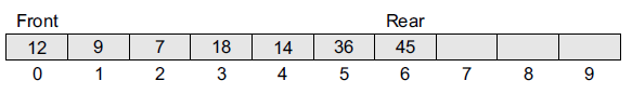
A queue is an ordered list in which all insertions can take place at one end called the rear and all deletions take place at the other end called the front.

A queue is a first-in, first-out (FIFO) data structure in which the element that is inserted first is the first one to be taken out.

Like stacks, queues can be implemented by using either arrays or linked lists.

Insert element into the Queue:

Here, front = 0 and rear = 5. If we want to add one more value to the list, say, if we want to

add another element with the value 45, then the rear would be incremented by 1 and the value

would be stored at the position pointed by the rear. Here, front = 0 and rear = 6.

Delete element from Queue: 

if we want to delete an element from the queue, then the value of front will be incremented.

Deletions are done only from this end of the queue.

However, before inserting an element in the queue, we must check for overflow conditions. An overflow occurs when we try to insert an element into a queue that is already full. A queue is full when rear = MAX – 1, where MAX is the size of the queue, that is MAX specifies the maximum number of elements in the queue. Note that we have written MAX – 1 because the index starts from 0.

Similarly, before deleting an element from the queue, we must check for underflow conditions.An underflow condition occurs when we try to delete an element from a queue that is already empty. If front = NULL and rear = NULL, then there is no element in the queue.

Linked Lists:

The major drawback of an array is that the number of elements must be known in advance. Hence an alternative approach was required. This give rise to the concept called linked list

   

Linked list is a dynamic data structure in which elements (called nodes) form a sequential list.

Here is that every node will have two parts: first part contains the information/data and the second part contains the link/address (pointer) of the next node in the list. Memory is allocated for every node when it is actually required. and will be freed when not needed.

The first node in the list is pointed by Head/Start/First. The last node in the list contains a NULL pointer to indicate that it is the end or tail of the list.

Advantage: Easier to insert or delete data elements

Disadvantage: Slow search operation and requires more memory space.

Trees:

A tree is a non-linear data structure. This structure is mainly used to represent data containing a hierarchical relationship between elements like family tree, organisation chart etc.

A tree is a finite set of one or more nodes such that:

(1) There is a specially designated node called the root.

(1) The remaining nodes are partitioned into n >= 0 disjoint sets T₁,..... Tn, where each of these sets is a tree. T₁,..... Tn are called sub-trees of the root.

The simplest form of a tree is a binary tree. A binary tree consists of a root node and left and right sub-trees, where both sub-trees are also binary trees. Each node contains a data element, a left pointer which points to the left sub-tree, and a right pointer which points to the right sub-tree.

The root element is the topmost node which is pointed by a ‘root’ pointer. If root = NULL then the tree is empty.

Here R is the root node and T1 and T2 are the left and right subtrees of R. If T1 is non-empty, then T1 is said to be the left successor of R. Likewise, if T2 is non-empty, then it is called the right successor of R.

Node 2 is the left child and node 3 is the right child of the root node 1. Note that the left sub-tree of the root node consists of the nodes 2,4, 5, 8, and 9. Similarly, the right sub-tree of the root node consists of the nodes 3, 6, 7, 10, 11, and 12.

Advantage: Provides quick search, insert, and delete operations

Disadvantage: Complicated deletion algorithm.

Graphs:

A graph is a non-linear data structure which is a collection of vertices (also called nodes) and edges that connect these vertices.

A node in the graph may represent a city and the edges connecting the nodes can represent roads.

A graph can also be used to represent a computer network where the nodes are workstations and the edges are the network connections.

Graphs do not have any root node. Rather, every node in the graph can be connected with every another node in the graph.

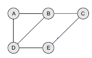
A graph G may be defined as a finite set. V of vertices and a set E of edges (pair of connected vertices). The notation used is as follows: Graph G (V, E). Consider the graph 

The set of vertices for the graph is V = (1, 2, 3, 4, 5). The set of edges for the graph is E {(1,2), (1,5), (1.3), (5,4),(4,3), (2.3)}

Advantage: Best models real-world situations.

Disadvantage: Some algorithms are slow and very complex.

OPERATIONS ON DATA STRUCTURES:

1. Creating. This is the first operation to create a data structure. This is just declaration and initialization of the data structure and reserved memory locations for data elements.

2. Inserting. Adding new records to the structure.

3. Deleting. Removing a record from the structure.

4.Updating. It changes data values of the data structure.

5. Traversing. Accessing each record exactly once so that certain items in the record may be processed. (This accessing or processing is sometimes called visiting the records.)

6. Searching. Finding the location of the record with a given-key value, or finding the locations of all records, which satisfy one or more conditions in the data. 

7. Sorting. Arranging the data elements in some logical order, i.e., in ascending and 

descending order 

8. Merging. Combine the data elements in two different sorted sets into a single sorted.

9. Destroying. This must be the last operation of the data structure and apply this 

operation when no longer needs of the data structure.

ABSTRACT DATA TYPE:

An abstract data type (ADT) is a data structure, focusing on what it does and ignoring how it does its job. (or) Abstract Data type (ADT) is a type (or class) for objects whose behavior is defined by a set of value and a set of operations.

Ex: stacks ADT and queues ADT. the user is concerned only with the type of data and the operations that can be performed on it.

• We can implement both these ADTs using an array or a linked list.

To understand the meaning of an abstract data type, we will break the term into ‘data type’ and ‘abstract’.

• Data type Data type of a variable is the set of values that the variable can take. We have already read the basic data types in C include int, char, float, and double.

When we talk about a primitive type (built-in data type), we actually consider two things: a data item with certain characteristics and the permissible operations on that data.

 For example, an int variable can contain any whole-number value from –32768 to 32767 and can be operated with the operators +, –, *, and /. 

    Therefore, when we declare a variable of an abstract data type (e.g., stack or a queue), we also need to specify the operations that can be performed on it.

• Abstract The word ‘abstract’ in the context of data structures means considered apart from the detailed specifications or implementation

In C, an abstract data type can be a structure considered without regard to its implementation.It can be thought of as a ‘description’ of the data in the structure with a list of operations that can be performed on the data within that structure.

For example, when we use a stack or a queue, the user is concerned only with the type of data and the operations that can be performed on it.

    They should just know that to work with stacks, they have push() and pop() functions available to them. Using these functions, they can manipulate the data (insertion or deletion) stored in the stack.

Advantage of using ADTs

• Modification of a program is simple, For example, if you want to add a new field to a student’s record to keep track of more information about each student, then it will be better to replace an array with a linked structure to improve the program’s efficiency.
• In such a scenario, rewriting every procedure that uses the changed structure is not desirable. Therefore, a better alternative is to separate the use of a data structure from the details of its implementation.

Differences between Array based and Linked based implementation